How To Get A Checkmark In Excel

Watch video – Insert and Use Checkmark Symbol in Excel

Below is the written tutorial, in example y'all prefer reading over watching the video.

In Excel, in that location are two kinds of tick marks (✓) that you can insert – a bank check mark and a checkbox.

And no… these are non the aforementioned.

Let me explain.

• Cheque Mark Vs Bank check Box
• Inserting Check Marker Symbol in Excel
  • Re-create and Paste the Check Marker
  • Utilize the Keyboard Shortcuts
  • Using the Symbols Dialog Box
  • Using the CHAR Formula
  • Using Autocorrect
  • Using Provisional Formatting to Insert Check Marker
  • Using a Double-Click (uses VBA)
• Formatting the Check Mark Symbol
• Format Bank check Mark / Cantankerous Mark Using Provisional Formatting
• Count Check Marks

Check Mark Vs Bank check Box

While a cheque mark and a checkbox may look somewhat like, these two are very different in the style it can be inserted and used in Excel.

A cheque mark is a symbol that you lot can insert in a cell (just like whatever text that you blazon). This means that when you copy the prison cell, you as well re-create the check marker and when you delete the prison cell, you also delete the cheque mark. Simply like regular text, you can format it by changing the color and font size.

A checkbox, on the other paw, is an object that sits above the worksheet. So when you place a checkbox above a cell, information technology's not a function of the prison cell but is an object that is over it. This means that if you delete the jail cell, the checkbox may not get deleted. As well, you can select a checkbox and elevate it anywhere in the worksheet (as it'due south not bound to the jail cell).

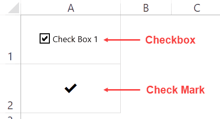
You will discover checkboxes being used in interactive reports and dashboards, while a checkmark is a symbol that yous may want to include every bit a office of the report.

A cheque mark is a symbol in the cell and a checkbox (which is literally in a box) is an object that is placed above the cells.

In this article, I volition merely be covering check marks. If you want to learn more about checkbox, hither is a detailed tutorial.

There are quite a few ways that you tin use to insert a check mark symbol in Excel.

Click here to download the example file and follow along

Inserting Check Marking Symbol in Excel

In this commodity, I will show you all the methods I know.

The method you apply would be dependent on how yous want to use the check marking in your work (equally y'all'll see later in this tutorial).

Permit'southward get started!

Copy and Paste the Bank check Mark

Starting with the easiest ane.

Since y'all're already reading this commodity, you lot can copy the below check mark and paste it in Excel.

To do this, re-create the check mark and go to the cell where yous want to copy information technology. Now either double-click on the cell or press the F2 key. This volition have yous to the edit fashion.

✔

Simply paste the check mark (Control + V).

One time you take the check mark in Excel, you can copy it and paste information technology as many times every bit you want.

This method is suited when you want to copy paste the bank check mark in a few places. Since this involves doing it manually, information technology's not meant for huge reports where you lot take to insert check marks for hundreds or thousands of cells based on criteria. In such a instance, it's better to utilize a formula (equally shown later in this tutorial).

Utilize the Keyboard Shortcuts

For using the keyboard shortcuts, you lot will accept to change the font of the cells to Wingdings 2 (or Wingdings based on the keyboard shortcut you're using).

Beneath are the shortcuts for inserting a bank check mark or a cantankerous symbol in cells. To use the below shortcuts, yous need to change the font to Wingdings 2.

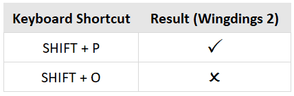
Beneath are some more keyboard shortcuts that you can use to insert check mark and cross symbols. To utilise the below shortcuts, you demand to alter the font to Wingdings (without the 2).

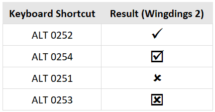
This method is best suited when you lot only desire a check mark in the cell. Since this method requires yous to change the font to Wingdings or Wingdings 2, it will not be useful if y'all want to have any other text or numbers in the aforementioned prison cell with the check mark or the cantankerous mark.

Using the Symbols Dialog Box

Another mode to insert a check marker symbol (or whatever symbol for that matter) in Excel is using the Symbol dialog box.

Hither are the steps to insert the bank check marking (tick mark) using the Symbol dialog box:

1. Select the prison cell in which you desire the check mark symbol.
2. Click the Insert tab in the ribbon.
3. Click on the Symbol icon.
4. In the Symbol dialog box that opens, select 'Segoe UI Symbol' every bit the font.
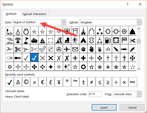
5. Scroll down till you find the check mark symbol and the double click on it (or click on Insert).

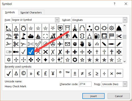
The higher up steps would insert one check mark in the selected cell.

If y'all want more than, simply copy the already inserted ane and apply it.

Notation that using 'Segoe UI Symbol' allows you to employ the bank check marker in any regularly used font in Excel (such as Arial, Time Now, Calibri, or Verdana). The shape and size may conform a lilliputian based on the font. This also means that you can have text/number along with the bank check mark in the same jail cell.

This method is a fleck longer merely doesn't require you lot to know any shortcut or CHAR code. One time y'all accept used it to insert the symbol, you can reuse that one past copy pasting it.

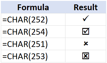
Using the CHAR Formula

You lot can use the CHAR office to return a check mark (or a cross marking).

The below formula would return a cheque marking symbol in the cell.

=CHAR(252)

For this to work, you need to catechumen the font to Wingdings

Why?

Because when you use the CHAR(252) formula, information technology would give you the ANSI character (ü), and so when yous change the font to Wingdings, it is converted to a bank check mark.

Y'all tin can utilize similar CHAR formulas (with different code number) to become another format of the bank check mark or the cross mark.

The real benefit of using a formula is when you lot use it with other formulas and return the check mark or the cross marker equally the result.

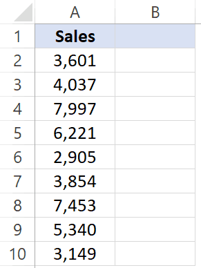
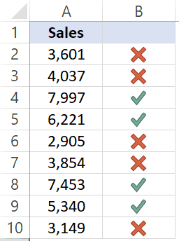
For example, suppose you have a dataset as shown below:

You can apply the beneath IF formula to get a check mark if the auction value is more than 5000 and a cross mark if it'south less than 5000.

=IF(A2>5000,CHAR(252),CHAR(251))

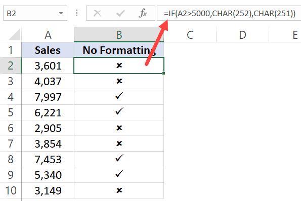
Retrieve, you need to catechumen the cavalcade font to Wingdings.

This helps you brand your reports a petty more than visual. It also works well with printed reports.

If you lot want to remove the formula and only keep the values, re-create the cell and paste it as value (right-click and choose the Paste Special and and then click on Paste and Values icon).

This method is suited when y'all want the check mark insertion to be dependent on cell values. Since this uses a formula, you can use it fifty-fifty when you have hundreds or thousands of cells. Also, since you demand to change the font of the cells to Wingdings, you can't have anything else in the cells except the symbols.

Using Autocorrect

Excel has a feature where information technology can autocorrect misspelled words automatically.

For example, type the word 'bcak' in a prison cell in Excel and see what happens. It will automatically correct it to the word 'back'.

This happens as there is already a pre-made list of expected misspelled words you're likely to blazon and Excel automatically corrects it for you.

Hither are the steps to utilize autocorrect to insert the delta symbol:

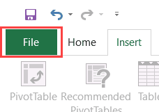
1. Click on the File tab.
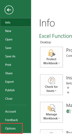
2. Click on Options.
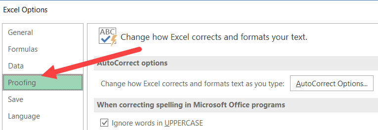
3. In the Options dialogue box, select Proofing.
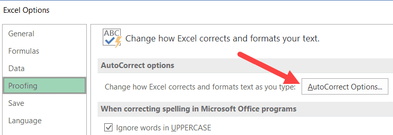
4. Click on the 'AutoCorrect Options' push button.
5. In the Autocorrect dialogue box, enter the following:
   • Supersede: CMARK
   • With: ✔ (y'all tin copy and paste this)
6. Click Add and so OK.

At present whenever you lot type the words CMARK in a cell in Excel, it volition automatically change it to a check mark.

Here are a few things y'all need to know when using the Autocorrect method:

• This is case sensitive. And so if you enter 'cmark', it will not get converted into the check mark symbol. You need to enterCMARK.
• This modify likewise gets applied to all the other Microsoft applications (MS Give-and-take, PowerPoint, etc.). So be cautious and choose the keyword that you are highly unlikely to use in any other application.
• If there is whatever text/number before/after CMARK, it will not be converted to the check mark symbol. For example, '38%CMARK' will non go converted, notwithstanding, '38% CMARK' will get converted to '38% ✔'

Related Tutorial: Excel Autocorrect

This method is suited when yous desire a ready reference for the check marking and you use it regularly in your work. So instead of remembering the shortcuts or using the symbols dialog box, you can rapidly utilise the shortcode name that you have created for bank check mark (or any other symbol for that affair).

Click here to download the example file and follow along

Using Conditional Formatting to Insert Bank check Marker

You tin use conditional formatting to insert a check mark or a cross mark based on the cell value.

For example, suppose you accept the data set as shown below and you want to insert a bank check mark if the value is more than 5000 and a cross marker if information technology's less than 5000.

Here are the steps to practice this using provisional formatting:

1. In cell B2, enter =A2, and so copy this formula for all cells. This will make sure that now you have the same value in the adjacent jail cell and if you modify the value in cavalcade A, information technology's automatically changed in column B.
2. Select all the cells in column B (in which you want to insert the cheque marker).
3. Click the Home tab.
4. Click on Provisional Formatting.
5. Click on New Rule.
6. In the 'New Formatting Dominion' dialog box, click on the 'Format Mode' drop downwards and click on 'Icon Sets'.
7. In the 'Icon Manner' driblet-down, select the manner with the check mark and cross mark.
8. Cheque the 'Show Icon only' box. This will ensure that simply the icons are visible and the numbers are hidden.
9. In the Icon settings. change the 'percentage' to the 'number' and brand the settings as shown below.
10. Click OK.

The above steps will insert a green bank check marker whenever the value is more than or equal to 5000 and a crimson cross mark whenever the value is less than 5000.

In this instance, I have only used these two icons, but you can also utilize the yellow exclamation mark as well if you want.

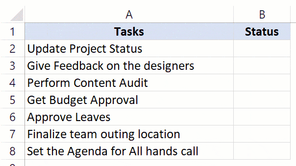
Using a Double-Click (uses VBA)

With a trivial flake of VBA code, you can create an awesome functionality – where it inserts a check marking equally presently every bit you lot double click on a prison cell, and removes it if you double click again.

Something as shown below (the carmine ripple indicates a double click):

To do this, you need to use the VBA double-click event and a simple VBA code.

But earlier I requite you the full code to enable double click, permit me quickly explicate what how VBA can insert a bank check mark. The beneath lawmaking would insert a check mark in cell A1 and change the font to Wingdings to make certain you run into the check symbol.

Sub InsertCheckMark() Range("A1").Font.Proper noun = "Wingdings" Range("A1").Value = "ü" Terminate Sub

Now I will employ the same concept to insert a bank check mark on double click.

Below is the code to do this:

Private Sub Worksheet_BeforeDoubleClick(ByVal Target As Range, Cancel As Boolean) If Target.Cavalcade = ii Then Abolish = True Target.Font.Proper noun = "Wingdings"     If Target.Value = "" Then         Target.Value = "ü"     Else         Target.Value = ""     End If End If Finish Sub

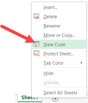
You need to copy and paste this code in the code window of the worksheet in which you lot need this functionality. To open the worksheet code window, left-click on the canvass proper name in the tabs and click on 'View Lawmaking'

This is a good method when you demand to manually scan a listing and insert check marks. Y'all tin can easily practice this with a double click. The best utilize case of this is when you lot're going through a list of tasks and accept to marking it every bit done or not.

Click here to download the example file and follow forth

Formatting the Check Marking Symbol

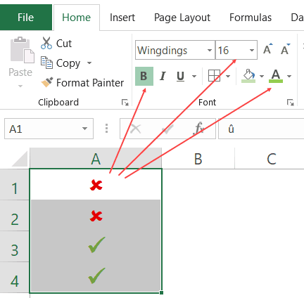
A bank check mark is just similar any other text or symbol that y'all utilise.

This means that yous can easily alter its color and size.

All you need to practice is select the cells that accept the symbol and apply the formatting such as font size, font color, and bold etc.

This way of formatting symbols is manual and suited simply when you have a couple of symbols to format. If y'all take a lot of these, information technology's meliorate to use conditional formatting to format these (as shown in the side by side department).

Format Check Marker / Cantankerous Mark Using Conditional Formatting

With conditional formatting, you lot tin format the cells based on what blazon of symbol it has.

Below is an example: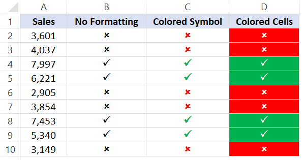

Column B uses the CHAR function to return a check mark if the value is more than 5000 and a cross mark if the value is less than 5000.

The ones in column C and D uses conditional formatting and await style meliorate as it improves visual representation using colors.

Let's come across how you tin practice this.

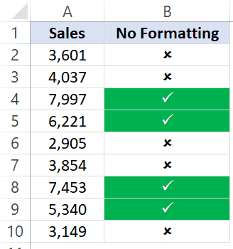
Below is a dataset where I have used the CHAR function to get the cheque mark or cross mark based on the prison cell value.

Below are the steps to color the cells based on the symbol it has:

1. Select the cells that have the check-marking/cantankerous-mark symbols.
2. Click the Habitation tab.
3. Click on Conditional Formatting.
4. Click on 'New Rule'.
5. In the New Formatting Rule dialog box, select 'Use a formula to decide which cells to format'
6. In the formula field, enter the following formula: =B2=CHAR(252)
7. Click the Format button.
8. In the 'Format Cells' dialog box, go to the Fill tab and select the greenish color.
9. Get to the Font tab and select color as white (this is to make sure your checkmark looks nice when the prison cell has a green background color).
10. Click OK.

Later the to a higher place steps, the data is going to await as shown below. All the cells that have the check marking will exist colored in green with white font.

Y'all need to repeat the aforementioned steps to now format the cells with a cantankerous mark. Change the formula to =B2=char(251) in step 6 and formatting in pace 9.

Count Bank check Marks

If you want to count the total number of check marks (or cross marks), you can do that using a combination of COUNTIF and CHAR.

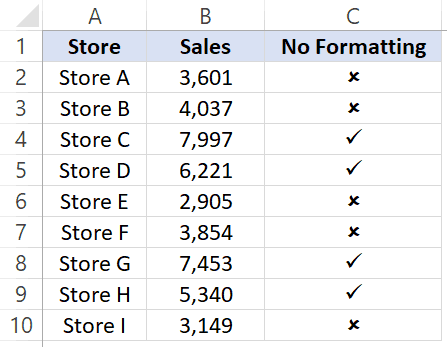
For example, suppose you have the information set as shown below and y'all desire to find out the total number of stores that have achieved the sales target.

Below is the formula that will give you the total number of check marks in column C

=COUNTIF($C$2:$C$x,CHAR(252))

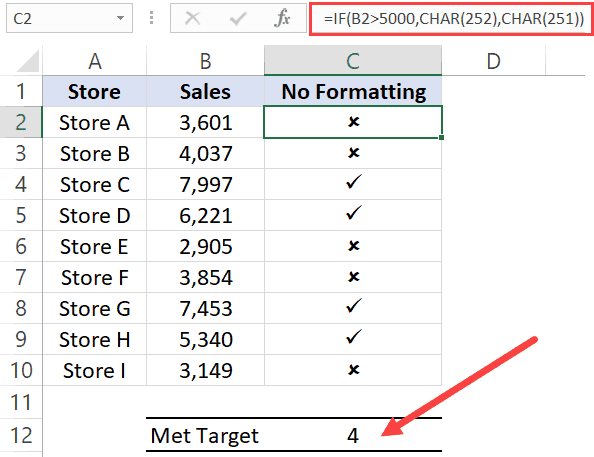
Annotation that this formula relies on you using the ANSI code 252 to become the check mark. This would work if y'all have used the keyboard shortcut ALT 0252, or take used the formula =Char(252) or accept copied and pasted the cheque mark that is the created using these methods. If this is not the case, so the higher up COUNTIF role is non going to work.

Yous May Also like the post-obit Excel tutorials:

• How to Insert Delta Symbol in Excel.
• How to Insert Degree Symbol in Excel.
• How to Insert a Line Break in Excel.
• How to Compare two columns in Excel.
• To-do List Excel Template.

Source: https://trumpexcel.com/check-mark/

Posted by: cooperevines1973.blogspot.com

Share this post